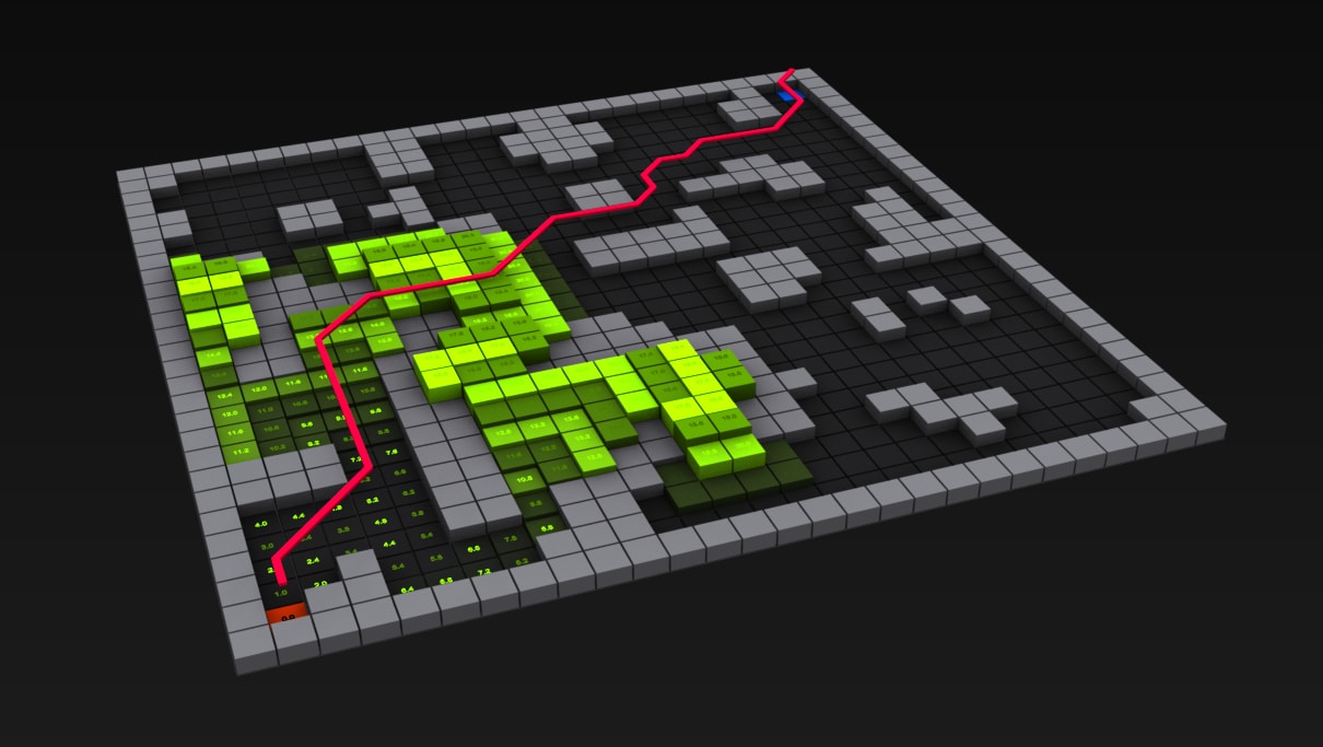
Essentially, a pathfinding algorithm attempts to find the "shortest" path, or the path with the lowest cost between two nodes on a graph. These algorithms play a vital part in modern technology, as they are integrated in common applications such as online map services and satellite navigation systems. Read more about pathfinding algorithms and graphs here.
This application was made to demonstrate how each algorithm works and performs. As a disclaimer, the cost of moving from one node to the next is one, and algorithms will prioritize a straight path over a path with many turns if it has the same cost. Take a look at all of the available algorithms in the next slide.
Next
×
The Pathfinding Algorithms and Heuristics
A quick description of each algorithm
Dijkstra's Algorithm: One of the most popular pathfinding algorithms. It considers weights of each visited node and guarantees the shortest path.
A* Pathfinding Algorithm: This is the best pathfinding algorithm that utilizes the cost of the path so far g(n){" "} and the estimate from the heuristic function h(n). It considers weights of each visited node and dguarantees the shortest path.
Greedy Best First Search: This algorithm utilizes a heuristic function h(n) to determine the next node to explore. It considers thee weights of each visited node but it does not guarantee an optimal solution.
Breadth First Search: This algorithm searches all of the nodes in the same depth before proceeding to the next depth level. This algorithm does NOT consider the weights of nodes, but will guarantee the shortest path.
Bidirectional Breadth First Search: This algorithm is essentially the same as breadth first search. However, instead of beginning the search at the start node, it begins the search at both the start and finish nodes.
Depth First Search: This algorithm is one of the worst pathfinding algorithms. It attempts to visit the "deepest" nodes first and backtracks once no other nodes can be visited. This algorithm does NOT consider the weights of the nodes and it does NOT guarantee the shortest path.
A quick description of each heuristic
Manhattan Distance: Uses the formula, d = |x1 - x2| + |y1 - y2| to give an estimate cost.
Euclidean Distance Uses the formula, d = √ (x1 - x2)2 + (y 1 - y2)2to give an estimate cost.
PreviousNext
×
Modifying the Grid
Besides changing the algorithms and heuristics, it is also possible to add obstacles to the grid. Obstacles will effectively increase the cost of the node and may cause the algorithm to take a different path. To add obstacles, simply select one on the navbar and left-click on the desired node, or left-click and drag the mouse across the desired nodes. For reference;
Blank nodes have a cost of 1
Goblins have a cost of 2
Ogres have a cost of 5
Witches have a cost of 10
Bears have a cost of 15
Dragons have a cost of 25
On top of manually adding obstacles, there are a few mazes and patterns that can be automatically generated. To add one to the grid, simply select one from the menu bar and it will be generated promptly. If needed, the simulation speed can also be modified in a similar fashion. Lastly, it is possible to change the location of the start and end nodes. To do so, simply click, hold, and drag the terminal nodes to the desired location.
PreviousNext
×
That's All Folks!
This concludes the tutorial for my pathfinding visualizer.
Have fun playing around with all of the different algorithms!
The source code for this visualizer can be found on my github.